Hyunoo's StudyNote

An obvious characteristic of time series data that distinguishes them from cross-sectional data is temporal ordering. In time series analysis, the past can affect the future, but not vice versa. Another difference between cross-sectional and time series data is randomness. In cross-sectional analysis, random outcomes are fairly straightforward. Randomness is justified by random sampling. However, randomness in time series data is justified naturally because the outcomes of time series variables are not foreknown.

Static Models

Suppose that we have time series data available on two variables, say y and z, where yt and zt are dated contemporaneously.

Static regression models are also used when we are interested in knowing the tradeoff between y and z.

Finite Distributed Lag (FDL) Models

In a finite distributed lag (FDL) model, we allow one or more variables to affect y with a lag.

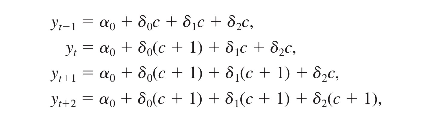
One example of FDL model is shown as

z is a constant, equal to c, in all time periods before time t. At time t, z increases by one unit to c + 1 and then reverts to its previous level at time t + 1.

To focus on the ceteris paribus effect of z on y,

From the two equations, yt - y(t-1) = δ0, which means that δ0 is the immediate change in y due to the one unit increase in z at time t. δ0 is usually called the impact propensity or impact multiplier. At the time t + 3, y has reverted to its initial level: y(t+3) = y(t-1).

------------------------------------------------------------------------------

We are also interested in the change in y due to a permanent increase in z. Before time t, z equals the constant c. At time t, z increases permanently to c + 1: zs = c, s < t and zs = c + 1, s >= t, setting the errors to zero.

With the permanent increase in z, after one period, y has increased by δ0 + δ1, and after two periods, y has increased by δ0 + δ1 + δ2. This shows that the sum of the coefficients on current and lagged z, δ0 + δ1 + δ2 is the long run change in y given a permanent increase in z and is called the long-run propensity(LRP) or long-run multiplier. For any horizon h, we can define the cumulative effect as δ0 + δ1 + δ2.....δh, which is interpreted as the change in the expected outcome h periods after a permanent, one-unit increase in x.

LRP =  δ0 + δ1 + δ2.....δh

Finite Sample Properties of OLS under Classical Assumptions

Assumption TS.1 Linear in Parameters

The stochastic process {(xt1, xt2.....,xtk, yt): t = 1, 2...., n} follows the linear model

yt = β0 + β1xt1 + β2xt2 ..... +  βkxtk + ut,

where {ut : t = 1, 2, ...., n} is the sequence of errors or disturbances. Here, n is the number of observations(time periods). xt1 = z1, xt2 = z2, ....

Assumption TS.2 No Perfect Collinearity

In the sample (and therefore in the underlying time series process), no independent variable is constant nor a perfect linear combination of the others.

Assumption TS.3 Zero Conditional Mean

For each t, the expected value of the error ut, given the explanatory variables for all time periods, is zero.

E(ut| xt1, xt2.... xtk) = E(ut|xt) = E(ut|X) = 0, t = 1, 2,.... , n

Assumption TS.3 implies that the error at time t, ut is uncorrelated with each explanatory variable in every time period. The fact that this is stated in terms of the conditional expectation means that we must also correctly specify the functional relationship between yt and the explanatory variables. If ut is independent of X and E(ut) = 0, then Assumption TS.3 automatically holds. (시간에 관계없이 항상) When this assumption holds, we say that xtj are contemporaneously exogenous and uncorrelated: Corr(utk, ut) = 0, for all j.

In a time series context, random sampling is almost never appropriate, so we must explicitly assume that the expected value of ut, is not related to the explanatory variables in any time period. (cross-sectional의 경우는 random sampling을 통해서 독립변수들과 ui 자동적으로 독립임을 증명해주었는데, 시계열 변수들은 직접 증명해주어야 함)

+ Anything that causes the unobservables at time t to be correlated with any of the explanatory variables in any time period causes Assumption TS.3 to fail. And in the social sciences, many explanatory variables may very well violate the strict exogeneity assumption. ex) the amount of labor input might not be strictly exogenous, as it is chosen by the farmer, and the farmer may adjust the amount of labor based on last year's yield.

Even though Assumption TS.3 can be unrealistic, we begin with it in order to conclude that the OLS estimators are unbiased. Assumption TS.3 has the advantage of being more realistic about the random nature of the xtj, while it isolates the necessary assumption about how ut, and explanatory variables are related in order for OLS to be unbiased.

Unbiasedness of OLS

Under assumptions TS.1 -3, the OLS estimators are unbiased conditional on X, and therefore unconditionally as well:

E(^βj) = βj, j = 0, 1, ....., k. 

Assumption TS.4 Homoskedasticity

Conditional on X, the variance of ut, is the same for all t : Var(ut|X) = Var(ut) = σ^2

This assumption requires that the unobservables affecting interest rates have constant variance over time.

경제지표 관련 회귀 선 내 ut에 interest rate가 t에 따라 변동하면 heteroskedasticity. 즉, constant해야 homoskedasticity.

Assumption TS.5 No serial Correlation

Conditional on X, the errors in two different time periods are uncorrelated: Corr(ut, us| X) = 0, for all t

≠ s. (Simply, Corr(ut, us) = 0m for all t ≠ s)

When this assumption is false, we say that the errors in this assumption suffer from serial correlation or, autocorrelation, because they are correlated across time. Consider the case of errors from adjacent time periods. Suppose that when u(t-1) > 0 then, on average, the error in the next time period, ut, is also positive. Then, Corr(ut, u(t-1)) > 0, and the errors suffer from serial correlation. In other words, TS.5 assumes nothing about temporal correlation in the independent variables.

Under Assumptions TS.1 through TS.5, the OLS estimators are the best linear unbiased estimators conditional on X.

Assumption TS.6 Normality

The errors ut, are independent of X and are independently and identically distributed as Normal(0,σ^2)

Resource : Jeffrey M. Woolderfige, "Introductory Econometrics : A Modern Approach 5th edition"

^log(wage) = .321 - .110female + .213married - .301female·married + other factors

Considering the interaction between female and married, we can append the interaction factor in the model.

Setting female = 0 and married = 0 corresponds to the group single men, which is the base group. Then we can find the intercept for married men by setting female = 0 and married = 1 in the model. (.321 + .213 = .534)

This model is just a different way of finding wage differentials across all gender marital status combinations. It allows us to easily test the null hypothesis that the gender differential does not depend on marital status.

Allowing for Different Slopes

log(wage) = (β0 + δ0female) + (β1 + δ1female)educ + u

               = β0 + δ0female + β1educ + δ1female·educ + u 

There are also occasions for interacting dummy variables with explanatory variables that are not dummy variables to allow for a difference in slopes. Continuing with the wage examples, suppose that we wish to test whether the return to education is the same for men and women, allowing for a constant wage differential between men and women. If we plug female = 0, then we find that the intercept for males is β0, and the slope on education for males is β1.  For females, we plug in female = 1; thus, the intercept for females is β0 + δ0, and the slope is β1 + δ1.  Therefore, δ0 measures the difference in intercepts between women and men, and δ1 measures the difference in the return to education between women and men. 

An important hypothesis is that the return to education is the same for women and men, which means that the slope of log(wage) with respect to educ is the same for men and women. A wage differential between men and women is allowed under this null, but it must be the same at all levels of education.

H0 : δ1 = 0

We are also interested in the hypothesis that average wages are identical for men and women who have the same levels of education. This means that δ0 and δ1 must both be zero under the null hypothesis. We use an F test to test H0 : δ0 = 0, δ1 = 0 

See ex 7.11 in the book, if you want to consider more than two interactions in one model.

Resource : Jeffrey M. Woolderfige, "Introductory Econometrics : A Modern Approach 5th edition"

Y = β0 + β1x + other factors,

under the condition of x1 is an ordinal variable.

- x1 has a range from zero to four, with zero being the worst and four being the best. 

The problem in this case is that the difference between four and three is not always the same as the difference between one and zero. In order to resolve it, we need to take a single credit rating and turn it into five categories.

Let x1 = 1 if x = 1, and x1 = 0 otherwise....

Then the model is established as

Y = β0 + δ1x1 + δ2x2 + δ3x1 + δ4x1 +  δ5x5 + other factors

Following our rule for including dummy variables in a model, we include four dummy variables because we have five categories. The omitted category here is a credit rating of zero, which is the base group.

If this model has a constant partial effect, there is one way to write the three restrictions that imply a constant partial effect. δ2 = 2*δ1, δ3 = 3*δ1, δ4 = 4*δ4

So the model can be reestablished as

Y = β0 + δ1(x1 + x2 + x3 + x4) + other factors

In some cases, the ordinal variable takes on too many values so that a dummy variable cannot be included for each value. For example, if one of the key IDV is the rank of the law school. Because each law school has a different rank, we clearly cannot include a dummy variable for each rank(너무 많아). If we do not wish to put the rank directly in the function, we can break it down into categories.

Resource : Jeffrey M. Woolderfige, "Introductory Econometrics : A Modern Approach 5th edition"

R-squared = 1 - (SSR/n)/(SST/n)

R-squared is simply an estimate of how much variation in y is explained by x1, ... xk in the population. A small R-squared does imply that the error variance is large relative to the variance of y, which means we may have a hard time precisely estimating the βj. However, the problem is that a large error variance can be offset by a large sample size.

But, the relative change in the R-squared when variables are added to an equation is very useful: the F statistic for testing the joint significance crucially depends on the difference in R-squared between the unrestricted and restricted models.

* an important consequence of a low R-squared is that prediction is difficult. Because most of the variation in y is explained by unobserved factors, and it's going to be hard in using the OLS equation to predict future outcomes on y given a set of values for the explanatory variables.

Adjusted R-squared

adjusted R-squared = 1 - [SSR/(n-k-1)]/[SST/(n-1)]
                            = 1 - ^σ^2/[SST/(n-1)]
                            = 1 - ( 1- R-squared)(n-1)/(n-k-1)
Define σy^2 as the population variance of y and let σu^2 denote the population variance of the error term, u. The population R-squared is defined as p^2 = 1 - σu^2/σy^2, this is the proportion of the variation in y in the population explained by the independent variables.

R-squared estimates σu^2 by SSR/n, which is biased. So why not replace SSR/n with SSR/(n-k-1)? Also, we can use SST(n-1) instead of SST/n.

The primary attractiveness of adjusted R-squared is that it imposes a penalty for adding additional independent variables to a model. The formula for adjusted R-squared shows that it depends explicitly on k, the number of independent variables. And the interesting point is that if we add a new independent variable to a regression equation, adjusted R-squared increases only if the t-statistic on the new variable is greater than one in absolute value. (An extension of this is that adjusted R-squared increases when a group of variables is added to a regression only if the F-statistic for joint significance of the new variables is greater than unity.)

Using Adjusted R-squared to choose between nonnested models

In some cases, we want to choose a model without redundant independent variables, and the adjusted R-squared can help with this.

ex) 

log(salary) = β0 + β1years + β2gamesyr + β3bavg + β4hrunsyr + u,

and

log(salary) = β0 + β1years + β2gamesyr + β3bavg + β4rbisyr + u

These two equations are nonnested models because neither equation is a special case of the other.

----------------------------------------------------------------------------------------------------------------------------------

In the case of nested models, one model(the restricted model) is a special case of the other model (the unrestricted model). One possibility of testing nested models is to create a composite model that contains all explanatory variables form the original models and then to test each model against the general model using the F test. The problem with this process is that either both models might be rejected or neither model might be rejected.

-----------------------------------------------------------------------------------------------------------------------------------

Comparing adjusted R-squared to choose among different nonnested sets of independent variables can be valuable when these variables represent different functional forms.

However, there is an important limitation in using adjusted R-squared to choose between nonnested models: we can not use it to choose between different functional forms for the dependent variable. ex) y or log(y)

Resource : Jeffrey M. Woolderfige, "Introductory Econometrics : A Modern Approach 5th edition"

^log(y) = ^β0 + ^β1*log(x1) + ^β2*X2

There are some advantages and disadvantages when we transform a linear regression function into a logarithmic functional form. When △DV per one unit IDV change is large, a logarithmic approximation is convenient to measure the change. We can estimate the percentage change of DV. 

Not only that, when y > 0, models using log(y) as the DV often satisfy the CLM assumptions more closely than models using the level of y. Strictly positive variables often have conditional distributions that are heteroskedastic or skewed. Another potential benefit of using logs is that taking the log of a variable often narrows its range. This is particularly beneficial when we measure large monetary values, such as firms' annual sales or baseball players' salaries. Narrowing the range of the DV and IDV can make OLS estimates less sensitive to outlying.

* There are some standard rules of thumb for taking logs.

- when a variable is a positive dollar amount, the log is often used. ex) wages, salaries, firm sales and firm market value

- population, the total number of employees, and school enrollment

- variables that are measured in years such as education, experience, tenure, age

- variables that are proportion or percent such as the unemployment rate, the participation rate

  -> in this case, we can interpret results with percentages point change.

One limitation of the log is that it cannot be used if a variable takes on zero or negative values. In cases where a variable y in nonnegative but can take on the value 0, log(1+y) is sometimes used. Technically, however, log(1+y) cannot be normally distributed. Another drawback of using log is that it is more difficult to predict the original variable. This model allows us to interpret log(y) not y.  

Resource : Jeffrey M. Woolderfige, "Introductory Econometrics : A Modern Approach 5th edition"

If we want to test whether a group of variables has no effect on the dependent variables, we use F-test.

A test of multiple restrictions is called a multiple hypotheses test or a joint hypotheses test. In this case, H0 constitutes exclusion restrictions.

the unrestricted model with k independent variables

the restricted model with k-q independent variables

H1 : H0 is not true

The way we proceed in testing H0 against H1 is to test the exclusion restrictions jointly.

Usually, the SSR from the restricted model is greater than the SSR from the unrestricted model, and the R-squared from the restricted model is less than the R-squared from the unrestricted model. What we need to decide is whether the increase in the SSR in going from the unrestricted model to the restricted model is large enough to warrant rejection of H0. In this case, we need a way to combine the information in the two SSRs to obtain a test statistic with a known distribution under H0.

For testing this hypothesis, we use the F statistic which is defined by

SSRr is the sum of squared residuals from the restricted model and SSRur is the sum of squared residuals from the unrestricted model.

q = numerator degrees of freedom = df(r) - df(ur)

n - k - 1 = denominator degrees of freedom = df(ur)

F is distributed as an F random variable with (q, n - k -1) degrees of freedom F ~ Fq,n-k-1

If H0 is rejected, then we say that Xk-q+1, ...., Xk are jointly statistically significant at the appropriate significance level. If the null is not rejected, then the variables are jointly insignificant, which often justifies dropping them from the model.

-----------------------------------------------------------------------------------------------------------------------------------

In testing general linear restrictions, the restrictions implied by a theory are more complicated than just excluding some independent variables. Let's assume that one of OLS slope estimators is 1 (ex. β1 = 1 and β2, β3, β4 = 0). In this situation, null hypothesis is defined by

H0 : β1 = 1 and β2, β3, β4 = 0

H1 : H0 is not true

The unrestricted model is

y = β0 + β1x1 + β2x2 + β3x3 + β4x4 + u

The restricted model is

y = β0 + x1 + u

y - x1 = β0 + u

β0s in the restricted model and unrestricted model are different.

The F statistic is defined by [(SSRr - SSRur)/SSRur][(n-q)/4]

In this testing, we cannot use the R-squared form of the F statistic for this example because the dependent variable in the restricted model is different from the one in the unrestricted model.

Resource : Jeffrey M. Woolderfige, "Introductory Econometrics : A Modern Approach 5th edition"