Resource: Robert H. Shumay & David S. Stoffer, 2016, 'Time Series analysis and its applications with R examples 4th edition'

Resource: Robert H. Shumay & David S. Stoffer, 2016, 'Time Series analysis and its applications with R examples 4th edition'

Resource: Robert H. Shumay & David S. Stoffer, 2016, 'Time Series analysis and its applications with R examples 4th edition'

In this section, we present the key concepts that are needed to apply the usual large sample approximations in regression analysis with time series data.


Stationary Stochastic Process


A stationary time series process is one whose probability distributions are stable over time in the following sense: if we take any collection of random variables in the sequence and that sequence ahead time periods, the joint probability distribution must remain unchanged.


In mathematical form, the stochastic process { xt : t = 1, 2, ..... } is stationary if for every collection of time indices 1 <= t1 < t2 < t3 .... < tm, the joint distribution of (xt1, xt2, ..... , tm) is the same as the joint distribution of (x(t+h), x(t+1 + h), ....., x(tm+h)) for all integers h >= 1. One implication (by choosing m = 1 and t1 = 1) is that xt has the same distribution as x1 for all t = 2, 3, .... which means that the sequence { xt : t = 1, 2, .... } is identically distributed. Furthermore, the joint distribution of (x1, x2) must be same as the joint distribution of (xt, x(t+1)) for any t >= 1. Again, this places no restrictions on how xt and x(t+1) are related to one another.


Requirement for Stationarity

1) the sequence {xt : t = 1, 2, ... } is identically distributed.

2) the nature of any correlation between adjacent terms is the same across all time periods. (including joint distribution)


Covariance Stationary Process

A stochastic process {xt : t = 1, 2, .....} with a finite second moment [E(xt^2) < ∞] is covariance stationary if

1) E(xt) is constant

2) Var(xt) is conatant

3) for any t, h >= 1, Cov(xt, x(t+h)) depends only h and not on t.


Covariance stationarity focuses only on the first two moments of a stochastic process: the mean and variance of the process are constant across time, and the covariance between xt and x(t+h) depends only on the distance between the two terms, h, and not on the location of the initial time period, t.


If a stationary process has a finite second moment, then it must be covariance stationary, but the converse is certainly not true. Sometimes, to emphasize that stationarity is called to strict stationarity to distinguish covariance stationarity which is a relatively weaker requirement. 


How is stationarity used in time series econometrics? On a technical level, stationarity simplifies statements of the law of large numbers and the central limit theorem. On a practical level, if we want to understand the relationship between two or more variables using regression analysis, we need to assume some sort of stability over time.


Weakly Dependent Time Series

Corr(xt, x(t+h)) -> 0 as h -> ∞


Weak dependence places restrictions on how strongly related the random variables xt and x(t+h) can be as the time distance between them, h, gets larger. A stationary time series process { xt: t = 1, 2,... } is said to be weakly dpendent if xt and x(t+h) are "almost independent" as h increases without bound.  Covariance stationary sequences can be characterized in terms of correlations: a covariance stationary time series is weakly dependent if the correlation between xt and x(t+h) goes to zero "sufficiently quickly " as h -> ∞. In other words, as the variables get farther apart in time, the correlation between them becomes smaller and smaller. Covariance stationary sequences where Corr(xt, x(t+h)) -> 0 as h -> ∞ are said to be asymtotically uncorrelated. 


Then, why is weak dependence important for regression analysis?

It replaces the assumption of random sampling in implying that the law of large numbers(LLN) and the central limit theorem(CLT) hold. The ost well known central limit theorem for time series data requires stationarity and some form of weak dependence: thus, stationary, weakly dependent time series are ideal for use in multiple regression analysis.


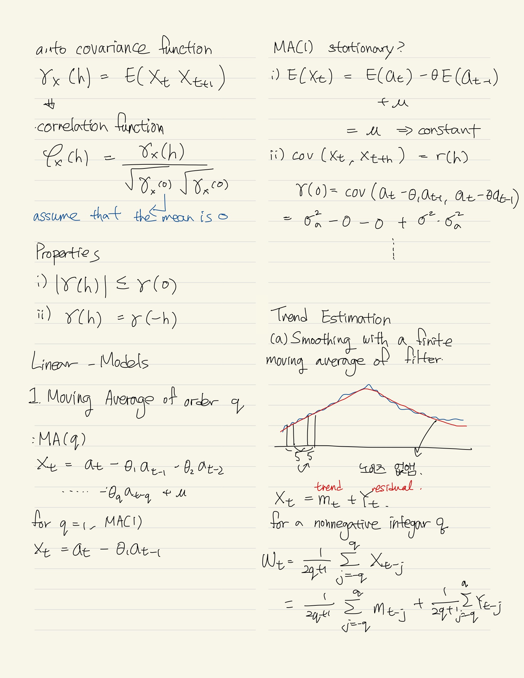
Moving average process of order one [MA(1)] : xt is a weighted average of et and e(t-1)


xt = et + αt*e(t-1), t = 1, 2, 3,.....,

where {et : t = 1, 2, 3....} is an i.i.d sequence with zero mean and variance σe^2.


Ma(1) process is weakly dependent. Adjacent terms in the sequence are correlated:

because x(t+1) = e(t+1) + α1*et, Cov(xt, x(t+1)) = α1, Var(et) = α1*σe^2.

Because Var(xt) = (1 + α1^2)*σe^2, Corr(xt, x(t+1)) = α1/(1+ α1^2).


 x(t+2) = e(t+2) + α1*e(t+1) is independent of xt because {et} is independent across t. Due to the identical distribution assumption on the et, {xt} is actually stationary. Thus, an MA(1) is a stationary, weakly dependent sequence and the law of large numbers and the central limit theorem can be applied to {xt}.


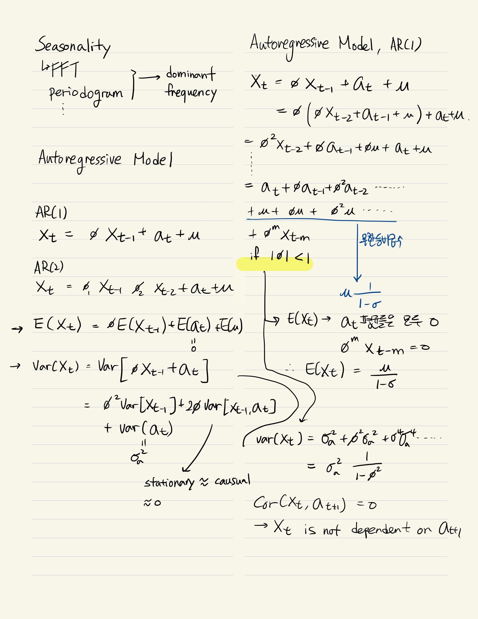
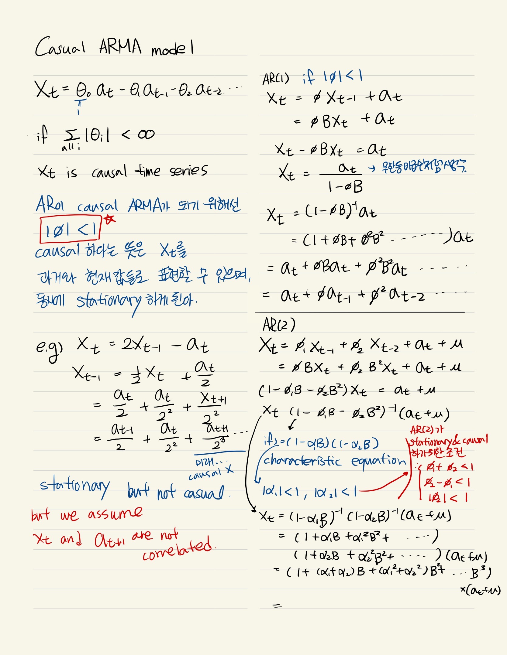
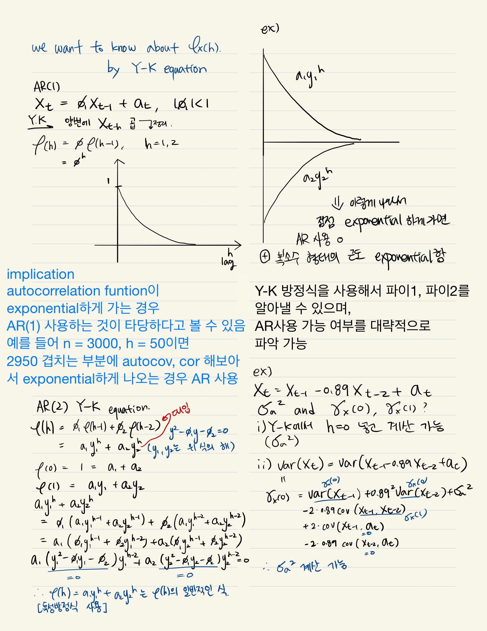
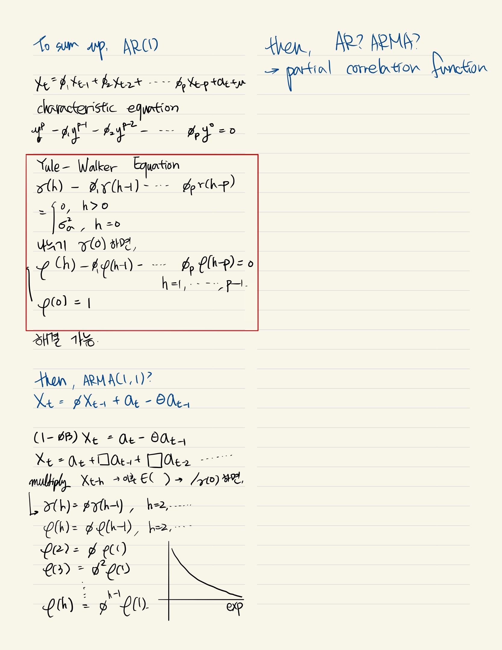
Autoregressive process of order one {AR(1)]


yt =ρ1*y(t-1) + et, t = 1, 2, ......

the starting point in the sequence is y0 (at t = 0), and { et : t = 1, 2, ... } is an i.i.d. sequence with zero mean and variance σe^2. The crucial assumption for weak dependence of as AR(1) process is the stability condition |ρ1| < 1. {yt} is a stable AR(1) process


To see that a stable AR(1) process is asymptotivally uncorrelated(weakly dependent), it is useful to assume that the process is covariance stationary. 

E(yt) = E(y(t-1)) - these are constant variables from requirement of covariance stationary.

and with ρ1 is not 1, this can only be possible if E(yt) = 0.

Var(yt) = ρ1^2Var(y(t-1)) + var(et)

and under covariance stationarity (Var(yt) = Var(y(t-1))),

σy^2 = ρ1^2*σy^2 + σe^2.


Since ρ1^2 < 1,

σy^2 = σe^2/(1-ρ1^2)


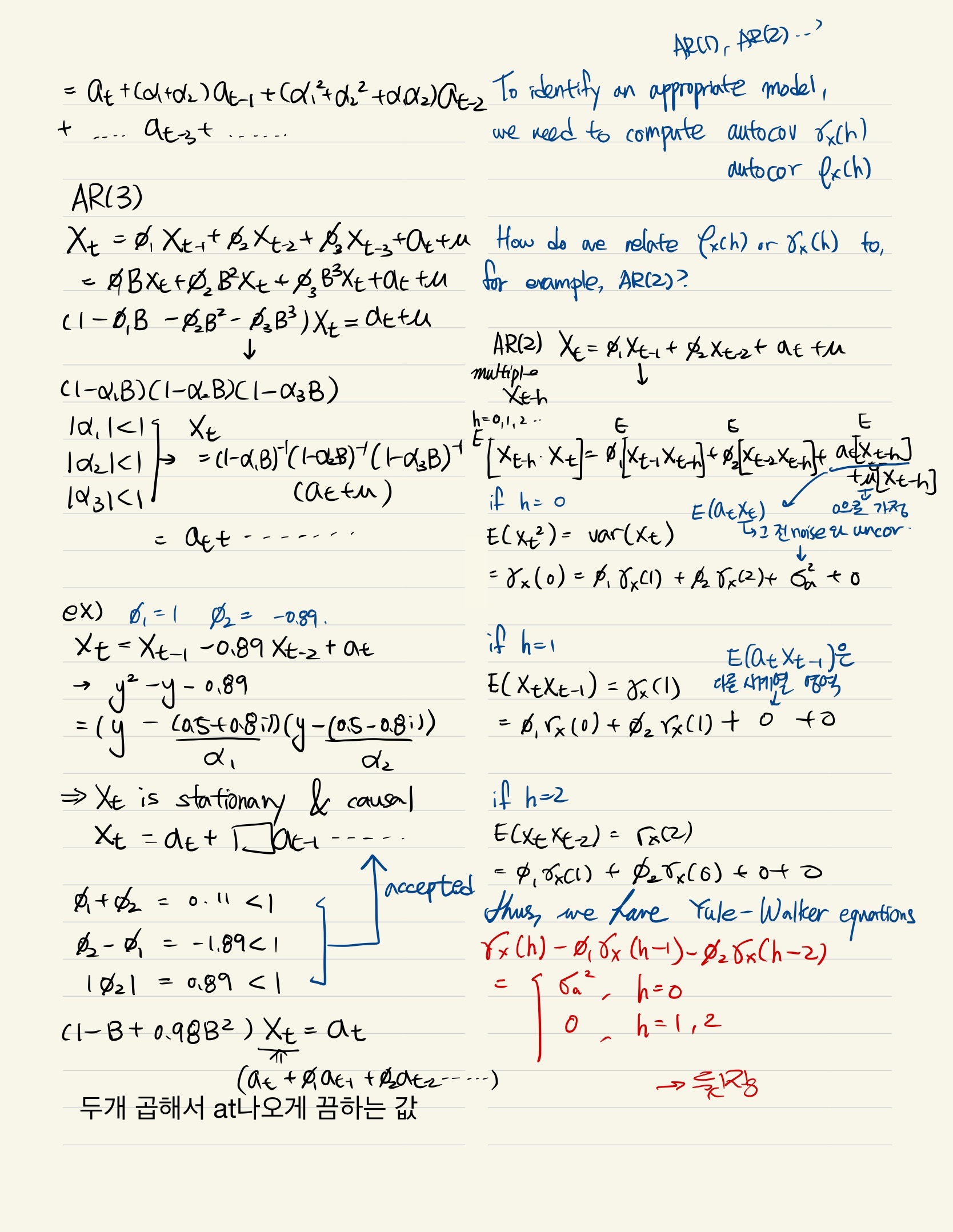
y(t+h) = ρ1y(t+h-1) + e(t+h) = ρ1(ρ1y(t+h-2) + e(t+h-1)+ + e(t+h)

         = ρ1^2*yt + ρ1^(h-1)*e(t+1)+.....p1*e(t+h-1) e(t+h)


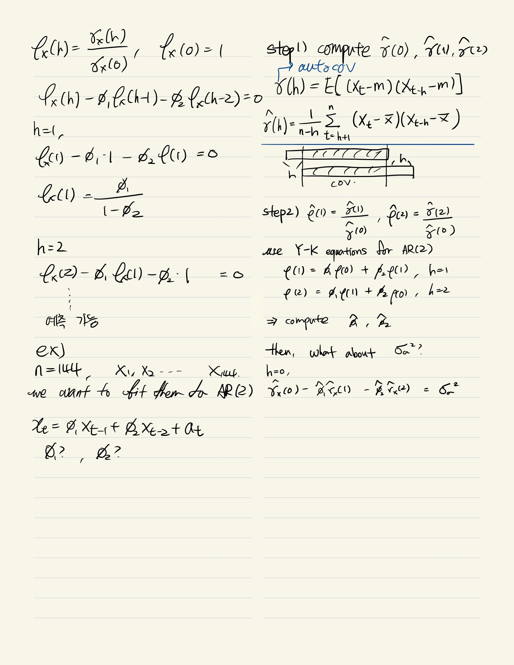
Due to E(yt) = 0 for all t, Cov(yt, y(t+h)) = E(yt, y(t+h)) =  ρ1^h*σy^2 (중간 과정 생략)


Corr(yt, y(t+h)) = Cov(yt, y(t+h))/(σy*σy) = ρ1^h

Corr(yt, y(t+1)) = ρ1


Corr(yt, y(t+h)) is important because it shows that, although yt and y(t+h) are correlated for any h >= 1, this correlation gets very small for large h : because |ρ1| < 1, ρ1^h -> 0 as h -> ∞. Thus, this analysis demonstrates that a stable AR(1) process is weakly dependent. 


Resource : Jeffrey M. Woolderfige, "Introductory Econometrics : A Modern Approach 5th edition"


Ignoring the fact two sequences are trending in the same or opposite directions can lead us to falsely conclude that changes in one variable are actually caused by changes in another variable. In many cases, two time series processes appear to be correlated only because they are both trending over time for reasons related to other unobserved factors. 

One popular formulation to capture this trend is


yt = α0 + α1*t + et, t = 1, 2,....,

where {et} is an independent, identically distributed(i.i.d.) sequence with E(et) = 0 and Var(et) = σ^2 (σ is the sigma of e).


We can write this mathematically by defining the change in et from period t-1 to t as Δet = et - e(t-1).

If Δet = 0, then Δyt = yt - y(t-1) = α1.


-----------------------------------------------------------------------------------------------------------------------------------


If {et} is an i.i.d, sequence, then {yt} is an independent, though not identically, distributed sequence. A more realistic characterization of trending time series allows {et} to be correlated over time, but this does not change the flavor fo a linear time trend. In fact, what is important for regression analysis under the classical linear model assumptions is that E(yt) is linear in t. 


----------------------------------------------------------------------------------------------------------------------------------


Many economic time series are better approximated by an exponential trend, which follows when a series has the same average growth rate from period to period.  For example, in the early years, we see that the change in imports over each year is relatively small, whereas the change increases as time passes. This is consistent with a constant average growth rate.

An exponential trend in a time series is captured by modeling the natural logarithm of the series as a linear trend (assuming that yt > 0):

log(yt) = β0 + β1t+ et, t = 1, 2,.....

yt itself shows an exponential trend: yt = exp(β0 + β1t+ et)


β1 can be interpreted as

Δlog(yt) = log(yt) - log(y(t-1)) ≈ (yt - y(t-1))/y(t-1)

(yt - y(t-1))/y(t-1) is also called the growth rate in y from period t-1 to t. To turn the growth rate tinto a percentage, we simply multiply by 100. 


Δlog(yt) = β1 if Δet = 0 for all t

In other words, β1 is approximately the average per period growth rate in yt

For example, if t denotes year and β1 = 0.39, then yt grows about 3.9% per year on average.


A Detrending Interpretation of Regressions with a Time Trend


^yt = ^β0 + ^β1*xt1 + ^β2*xt2 + ^β3*t


(Setting ^β3*t as a variable which considers time series changes so that other variables can show their changes regardless of time series changes)

(^β3*t값에 시간에 관한 모든 변화를 통제하게 하여, 다른 변수들은 변수 고유의 변화(시간 변화와 독립되어)만 보여줄 수 있게 함) = detrending


We can extend the results on the partialling out interpretation of OLS to show that ^β1, and ^β2 can be obtained as follows.

1) Regress each of yt, xt1, and xt2 on a contant and time trend t and save the residuals.


Thus, we can think of  ''y as being linearly detrended. In detrending yt, we have estimated the model

yt = α0 + α1t + et


the residuals from this regression, ^et = ''yt, have the time trend removed (at least in the sample). 


2) Run the regression of ''y on ''xt1, ''xt2


(No intercept in necesary, but including an intercept affects nothing: the intercept will be estimated to be zero.) This regression exactly yields ^β1 and ^β2 from ^yt = ^β0 + ^β1*xt1 + ^β2*xt2 + ^β3*t.

This means that the estimated of primary interest, ^β1 + ^β2, can be interpreted as coming from a regression without a time trend, but where we first detrend the dependent variable and all other independent variables.


Resource : Jeffrey M. Woolderfige, "Introductory Econometrics : A Modern Approach 5th edition"

ex) time series linear regression model with quarterly data 

log(Mt) = α0 + δ0log(GDPt) + δ1log(GDP(t-1))+ δ2log(GDP(t-2)) + δ3log(GDP(t-3)) + δ4log(GDP(t-4)) + ut


The impact propensity in this equation, δ0 is also called the short-run elasticity: it measures the immediate percentage change in money demand given a 1% increase in GDP. The long-run propensity, δ0 + δ1 + δ2 + ... + δ4, is called the long-run elasticity. It measures the percentage increase in money demand after four quarters given a permanent 1% increase in GDP.


-----------------------------------------------------------------------------------------------------------------------------------


Binary explanatory variables are the key component in what is called an event study. In an event study, the goal is to see whether a particular event influences some outcome. 


log(Mt) = α0 + δ0log(GDPt) + δ1log(GDP(t-1))+ δ2log(GDP(t-2)) + δ3log(GDP(t-3)) + δ4log(GDP(t-4)) + β1dt + ut


dt is a dummy variable indicating when the event occurred. For example, if the firm is an airline, dt might denote whether the airline experienced a publicized accident or near accident during week t. Sometimes, multiple dummy variables are used.


-----------------------------------------------------------------------------------------------------------------------------------

Index number typically aggregates a vast amount of information into a single quantity. It is often used in time series analysis, especially in macroeconomic applications. 

Base Period and the base value is defined as a period that is denoted as standard or base time of index number.

p360 - comparison between nominal and real variables (명목, 실질 변수 차이 계산)


Resource : Jeffrey M. Woolderfige, "Introductory Econometrics : A Modern Approach 5th edition"

+ Recent posts